Single crystal sample

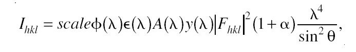
The integrated intensity I of a particular reflection measured in a TOF neutron diffraction experiment can be written as a function of the wavelength and the Bragg angle:

where h, k, l are the Miller indices designating the Bragg peaks, and the wavelength dependent correction factors are in the order given above: the incident
spectral neutron flux, the detector efficiency, the absorption correction, the extinction correction, and alfa= I_TDS/I_Bragg, the thermal diffuse scattering (TDS) correction.
( J. Peters and W. Jauch, Science Progress (2002), 85 (4), 297–317).
In this module we can treat the extinction, TDS correction by combining a normalisation factor, d-spacing spread or by a reflection dependent coefficient multiplying Fhkl² in the structure factor file.

Parameter descriptions

Parameter	Description	Command Option
parameter file	in this file are given: reciprocal unit vectors, normalisation, absorption, sample position, etc (see below)	-P
structure factor file	each line contains: h k l Fhkl² (see below)	-S
d-spacing distribution	options 1: Lorentzian, 2: Gaussian distributions, functions describing the d-spacing probability distribution with maximum at the nominal value (for the exact nominal value ideal reflectivity = 1., see also normalisation)	-o
d-spacing spread	gives FWHM/d-spacing, the relative 'thickness' of the Ewald sphere i.e. a small variation of the lattice constant which is same in each direction, silicon ~ 0.0001=0.01%	-d
reciprocal unit vectors A, B, C [1/A]	x,y,z components of the reciprocal unit vectors A, B, C defined in the sample frame	parameter file
normalisation [arb.u.]	normalisation factor containing for example the number density	parameter file
absorption [1/cm/A]	attenuation due to absorption within the sample per wavelength	parameter file
position X,Y,Z [cm]	coordinates of the sample centre	parameter file
phi(Z), chi(X), omega(again Z) [deg]	rotation angles of sample i.e. the reciprocal unit vectors around the Z, X and again Z axes	parameter file
sample geometry	sample shape options: 'cub', 'cyl'inder (vertical), 'ball'	parameter file
thickness or diameter, height, width [cm]	rectangular sample dimensions in x,y,z directions (sample frame)	parameter file
output angle horizontal, vertical [deg]	a frame rotation about the Z axis and then a rotation about the (new)Y axis defines a new orientation for the neutrons written to the output	parameter file

The parameter file contains in the first 3 lines the
reciprocal lattice vectors, and you can give a normalisation containing the
number denstity or other factors.

Example:

1.2892     0       0        recipr. unit v. A X [1/A], recipr. unit v. A Y [1/A], recipr. unit v. A Z [1/A]
0          1.2892 0        recipr. unit v. B X [1/A], recipr. unit v. B Y [1/A], recipr. unit v. B Z [1/A]
0          0       1.8982 recipr. unit v. C X [1/A], recipr. unit v. c Y [1/A], recipr. unit v. C Z [1/A]
1          0.01            normalisation [a.u.], absorbtion [1/cm/A]
900        0       0        position X [cm], position Y [cm], position Z [cm],
30       -15       0        phi(Z) [deg], chi(X) [deg], omega(Z) [deg]
cub                sample geometry: 'cub', 'cyl'inder, 'ball'
1          1       1        thickness or diameter [cm], height [cm], width [cm]
109.3     20.7            output angle horiz. [deg], output angle vert. [deg]

VITESS rotation convention: Smaller index axis rotated towards higher index axis is positive!

The structure factor file contains

no. refl    h     k     l     Fhkl²

in each line (Debay-Waller factor can be included here).
All incoming trajectories will sample each reflection and the successful ones are written out i.e. number of incoming trajectories will be larger than the number of incoming trajectories.
The third coordinate 'colour' will contain which reflection has happened (no.refl), this can be seen if you use 'writeout' to view the ASCII output (as in the example, but for longer runs do not forget
to cancel 'writeout' to save memory and computing time).

Example:

1 14 -11 -1 0.08057
2 15 -11 -1 0.00616
3 16 -11 -1 0.02162
4 17 -11 -1 0.01906
5 18 -11 -1 5.35824E-5
6 12 -10 -1 5.929E-7
7 13 -10 -1 0.00652
8 14 -10 -1 0.00228
9 15 -10 -1 0.49332
10 17 -10 -1 7.66736E-4
11 18 -10 -1 0.00165
12 19 -10 -1 5.67392E-4

Back to VITESS overview
vitess@hmi.de

Last modified: Wed Apr 2 18:53:44 MEST 2003, G. Zs.